Rethinking SETI Part 2: Who Can See Us?

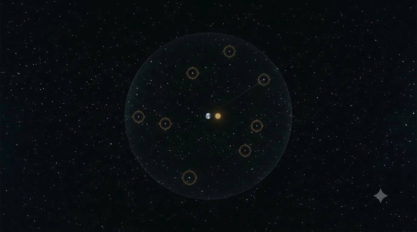
The classic SETI question is where transmitters might be. It ranges over the whole galaxy, it has no natural boundary, and no amount of null result finishes it — sixty-five years of radio searching have covered about six parts in a billion billion of one deliberately broad fiducial haystack, which is another way of saying the field has never been in a position for silence to mean anything.¹

There is a smaller question with a computable answer. Instead of asking where a transmitter could be, ask who has had the means and the time to notice Earth and answer.

Part 1: The Beacons Worth Building prices the transmitters that either of the two motives for building one — being heard, and being answered — would actually fund, and the catalog comes out shaped like a barbell: the money goes to the two ends of the design space, and the middle — the moderate-range, untargeted, continuous carrier that classic SETI implicitly hunted — is what nobody builds. This piece takes the near end of that barbell. Part 3: Looking Afar takes the far end.

The near end is the technosignature-targeted beacon: a transmitter parked on a world whose industry the builder has already watched appear. In Part 1’s catalog it is the first purchase of both buyers — the message broadcaster’s cheapest recipient and the reply-seeker’s only design with plausible positive net present value — because everything about it is local: it fires only at a target already confirmed to host a listener, it runs for a century instead of a hundred million years, and the geometry that makes it affordable also caps how far away its target can be. Its once-companion, a targeted beacon cued by biosignatures alone, does not survive Part 1’s pricing: life precedes listening by something like a hundred million years, no machine outlives that wait, and a builder holding a biosignature catalog spends it on the sweep schedule of a galactic-range beacon instead. Biosignatures still matter in this piece, but in a different role — not as the cue for a transmitter, as the cue for the watching the surviving design requires.

That exclusion rides on Part 1’s most contestable fiducial, the lifetime ceiling, and Part 1 names the published model that refuses it: Zuckerman’s purposely communicative builder, millions of years old, parks continuous transmitters on the few hundred living worlds within 200 parsecs and rides out the emergence lag.² The wager itself is argued there; what matters here is what his side of it does to this piece’s geometry. A builder that has watched Earth live for two billion years never waited for our onset, so the handshake radius dissolves, and the signal, if it exists, is arriving now, continuously, from solar-type stars at distances these lists never reach. The consolation is that the revived design is the cheapest on the board to constrain — a beacon bright enough to close Zuckerman’s link is bright enough to appear in sky surveys that were never looking for it — and the audit below collects that constraint.

The design implies two questions, asked from the receiving end. Who has had the means and the time to catch Earth’s technosignatures and answer? And, among those, who was already watching when the signature appeared? The first question is a computation over onset epochs and receiver models. The second is a prior, and transit geometry supplies it, because the stars that see Earth cross the Sun have held the cheapest possible read on our atmosphere for as long as it has carried oxygen. Both questions are close relatives of Eamonn Kerins’s mutual detectability criterion, that a transmitter should ask what the other party is in a position to infer,³ and of Amri Wandel’s argument that a civilization would restrict its attention to worlds already showing technology rather than mere biology.⁴ Two answers fall out. The lists are short enough to search to completion, which makes this one of the few places in SETI where a null result would constrain something other than our own diligence. And their size depends less on Earth than on the telescope assumed at the far end: across published receiver models, the count of possible responders moves by two orders of magnitude.

Three Nested Radii

Most discussions of Earth’s visibility collapse three different quantities into one. Separating them is the whole of the argument.

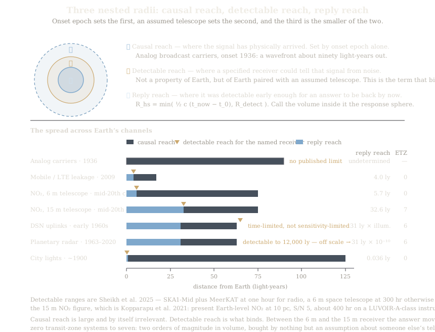
Causal reach is where a signal has physically arrived. It is set by onset epoch and nothing else. Earth’s first high-power broadcast carriers date from the 1930s, so a wavefront carrying them has swept about ninety light-years.

Detectable reach is where a specified receiver could distinguish that signal from noise. It depends on the emitted power, the beam, the propagation losses, and the aperture and integration time at the far end. It is almost always far smaller than the causal reach, and it is not a property of Earth alone: it is a property of Earth paired with an assumed telescope.

Reply reach is where the signal was detectable early enough for an answer to have returned. A world becomes conspicuous at epoch $t_0$; an observer at distance $d$ learns of it at $t_0 + d/c$; its reply arrives at $t_0 + 2d/c$. For that to be in our past, $d$ must be under half the light-age of the technosignature. The reply reach is therefore

$$R_{\text{reply}} = \min\!\left( \tfrac{1}{2}\,c\,(t_{\text{now}} - t_0),\; R_{\text{detect}} \right),$$

the smaller of a time limit and a sensitivity limit. Part 1 derived the same quantity from the transmitter’s side and called it the handshake radius; this piece reads it from the receiving end, as a reply radius, and calls the volume inside it the response sphere.

The distinction matters because the two terms bind under different circumstances and the answer changes by more than an order of magnitude depending on which one does. Almost every published statement about Earth’s radio bubble quotes the causal reach. Almost every useful statement about who could answer requires the other two.

A refinement follows from the geometry and is easy to miss. An observer whose reply arrives today transmitted $d$ years ago, and at that moment was looking at Earth as it was $2d$ years ago. The technosignature that matters is the one Earth emitted at $t_{\text{now}} - 2d/c$, not the one it emits now. For channels that have been growing this makes the sphere smaller than the naive calculation; for channels that peaked decades ago and have since declined, it makes the sphere larger. Either way the amplitude has to be evaluated at the retarded epoch.

How Conspicuous Is Earth?

Sheikh and colleagues recently did the necessary accounting, computing detection ranges for a dozen of Earth’s technosignatures against a single consistent set of present-day instrument assumptions.⁵ The results span thirteen orders of magnitude, and the ranking is not the one intuition supplies.

The ranges below all assume the same present-day receiver suite — an SKA-class array for the radio channels, a six-meter space telescope for the rest — with the particulars in the table notes. Our city lights reach 0.036 light-years, which does not clear the inner Oort cloud, and that figure is for a resolved urban fraction under a 300-hour stare. A single city’s heat island, taken as one JWST/MIRI pixel, reaches $4.7\times10^{-4}$ light-years; integrated over the disk, Earth’s waste heat is buried under natural ten-micron variability by a factor of fifty and is not detectable at all. Aggregate mobile-network leakage, modeled as 4 GW of LTE, reaches four light-years. Atmospheric nitrogen dioxide reaches 5.7 light-years, and that calculation uses the 1980 peak abundance of 113 parts per billion rather than today’s.

A single channel dwarfs the rest. Arecibo’s planetary radar radiated an effective 20 terawatts and would be detectable across twelve thousand light-years. It was also a two-arcminute beam, pointed north of the celestial equator near the ecliptic, transmitting perhaps one percent of the time, which puts the joint illumination probability for an observer who does not already know when to look at order $10^{-10}$. That duty-cycle arithmetic is mine, since nobody publishes radar duty cycles, and it is the listener-burden problem aimed back at us. On 1 December 2020 the platform fell into the dish. Goldstone’s radar survives at roughly an order of magnitude fainter.

The Deep Space Network sits between the two extremes and is usually left out of these inventories. Its spacecraft uplinks radiate about 965 MW effective and reach 65 light-years against the same SKA-class receiver. They are also beamed and aimed along the ecliptic at spacecraft, and the duty cycle — for years the unpublished number in this channel — now has a measurement: Fan, Wright and Lazio mined twenty years of public DSN scheduling logs and found the transmissions so concentrated toward the ecliptic that the average duty cycle toward the Earth Transit Zone runs twenty times the average across all ecliptic latitudes, and an observer along the Earth–Mars line at conjunction would have had a 77% chance of catching an uplink across the two decades logged.⁶ Earth’s brightest sustained beamed emission preferentially illuminates the one band of sky this piece will argue is most likely to be watching — a favor the transit-zone section below collects.

The channel table

Putting onset epochs against detection ranges gives the reply radius for each channel. Onsets are dated below; the causal column is $c(t_{\text{now}} - t_0)$ and the reply column is the smaller of half that and the detectable range.

Channel	Onset epoch	Causal reach	Detectable range	Time-limited radius	Reply radius	Transit-zone systems in range
Analog broadcast carriers	1936	~90 ly	not published	~45 ly	undetermined	undetermined
Mobile-network leakage	2009	~17 ly	4.0 ly (SKA-class)	~8.5 ly	4 ly	0
Atmospheric NO₂, 6 m	mid-20th c.	~75 ly	5.7 ly (300 hr)	~38 ly	5.7 ly	0
Atmospheric NO₂, 15 m	mid-20th c.	~75 ly	32.6 ly (400 hr)	~38 ly	32.6 ly	7
DSN spacecraft uplinks	early 1960s	~63 ly	65 ly (SKA-class)	~31 ly	31 ly × illum. prob.	6
Planetary radar	1963–2020	~63 ly	12,000 ly	~31 ly	31 ly × $10^{-10}$	6
City lights	~1900	~125 ly	0.036 ly	~63 ly	0.036 ly	0
Urban heat islands	~1900	~125 ly	$4.7\times10^{-4}$ ly	~63 ly	$4.7\times10^{-4}$ ly	0

Sources and receiver models: mobile leakage, NO₂ at six meters, radar, DSN, city lights and heat islands are Sheikh et al.’s Table 2 values, computed against SKA1-Mid plus MeerKAT at one hour for radio and a six-meter space telescope at 300 hours for the rest.⁵ The fifteen-meter NO₂ figure is Kopparapu et al.’s: present Earth-level NO₂ on an Earth analogue around a Sun-like star at 10 parsecs, detected at signal-to-noise 5 in about 400 hours by a LUVOIR-A-class instrument.⁷ Onset dates: first commercial radio broadcast 1920, BBC high-power television 1936, first commercial LTE network December 2009 with global deployment 2012–2014, Arecibo planetary radar from 1963 to its collapse in December 2020. The final column counts stellar systems currently in the Earth Transit Zone — the geometric filter introduced below — that fall inside each channel’s reply radius.

Most of the work in that table is done by three rows, and one of them is a hole.

The analog carriers are the hole. They are the origin of the “hundred-light-year radio bubble” that appears in every popular account, and no present-day-instrument detection range for them has been published, because Sheikh et al. modeled contemporary Earth and the high-power analog carriers were switched off in the United States in June 2009 and across the United Kingdom’s regional switchover between 2007 and 2012. The bubble exists as causal reach. Whether anything inside it was detectable is not established, which is why that row is blank. It is also the row where the retarded-epoch correction does real work: any observer far enough away that a reply could only now be arriving was watching the analog era at full strength, not today’s quiet spectrum.

The two NO₂ rows are the interesting pair, because they differ only in the size of the observer’s telescope and they differ by a factor of six in radius and by two hundred in volume. Which of them is right is not a fact about Earth.

One cross-check against Part 1 is worth making explicit, because it cuts. The trigger that fires the targeted beacon is most naturally a mid-infrared observation — industrial halocarbons between eight and twelve microns, waste heat at ten — and the mid-infrared rows of this table are its weakest. A single urban heat island reaches $4.7\times10^{-4}$ light-years, Earth’s disk-integrated waste heat is buried under natural ten-micron variability by a factor of fifty, and the halocarbons have no published detection range in transit geometry at all, for reasons the watcher-prior section below takes up. Whatever else Earth is, it is not conspicuous in the band a technosignature-cued builder would most naturally watch. This does not weaken the design, which fires on any confirmed technosignature rather than specifically a chemical one, but it relocates the burden: whatever triggered a beacon aimed at us is far more likely to be leakage or a beamed uplink than our chemistry — a second route to the conclusion the missing transmission forecast reaches below.

The Response-Sphere Census

Within the reply radii above, how many stars are there? The response sphere requires no transit geometry, since direct imaging and leakage interception work from any direction, so this is the plain local stellar census.

Radius	Stellar systems	Individual stars	Basis
4 ly	1	3	direct (α Centauri at 4.37 ly, just out)
5.7 ly	3	5	direct
10 ly	7	11	direct
20 ly	81	111	direct
25 ly	~120	~170	scaled
32.6 ly (10 pc)	269	370	scaled from Reylé density8
40 ly	~500	~690	scaled
50 ly	~970	~1,340	scaled

Scaled rows use Reylé et al.’s local densities of 0.089 stars and roughly 0.064 stellar systems per cubic parsec.⁸ Their direct ten-parsec census counts more, 339 systems and 540 objects, because it includes brown dwarfs; the scaled figures above are stellar. The twenty-light-year sphere is a local overdensity, so its direct count exceeds the density scaling, and Poisson noise on the inner spheres runs at ten percent or worse.

The census is the denominator. Under the fifteen-meter NO₂ model, the set of stars that could have read Earth’s industrial chemistry and replied by now is about 270 systems. Under the six-meter model it is three. Under the mobile-leakage model it is one, and that one is Alpha Centauri at 4.37 light-years, which is outside the 4.0-light-year detection radius, so it is zero.

That spread is the central result here, and it should be stated without decoration: the size of the population that could have answered us is set by an assumption about somebody else’s telescope, and it varies by two orders of magnitude across published receiver models. Any claim about the response sphere that does not name its receiver is not a claim.

The Earth Transit Zone as a Watcher’s Prior

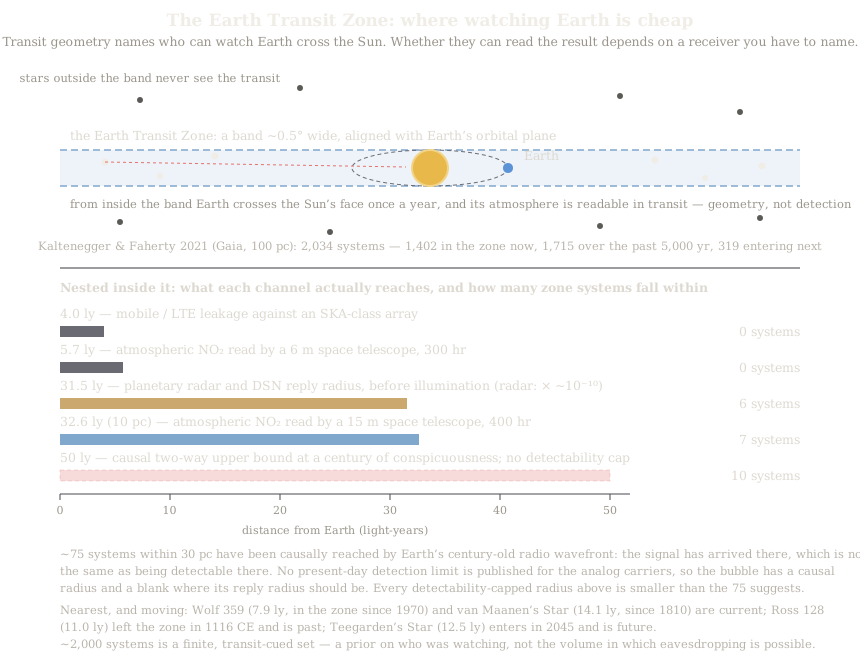
Transit geometry is the sharpest observing constraint available, because transit visibility is a strict geometric condition. In 2021 Lisa Kaltenegger and Jackie Faherty used Gaia astrometry to compute which stars occupy, or have occupied, the thin band of sky from which Earth can be seen crossing the Sun.⁹ Their catalog holds 2,034 systems within 100 parsecs: 1,402 in the zone now, 1,715 that have held the vantage at some point in the past five thousand years, and 319 entering over the next five thousand. Applying a 25% occurrence rate for rocky habitable-zone planets to the sample gives 508 candidate worlds that could both see Earth transit and plausibly host an observer.

What the zone is not is the complete set of observers capable of detecting Earth. Direct imaging characterizes a planet from any viewing geometry, and it is the method behind both NO₂ figures in the channel table. Leakage can be intercepted from any sufficiently nearby direction. And transit geometry by itself guarantees nothing about detectability, since seeing Earth cross the Sun is not the same as resolving oxygen or nitrogen dioxide in the transmission spectrum with the instrument you happen to own. The zone is a finite, high-priority, transit-cued subset. It is not the volume in which eavesdropping is physically plausible, and treating it as though it were confuses a geometric convenience with a detectability limit.

What the zone is, under Part 1’s economics, is the answer to a question about attention. The technosignature trigger’s real cost is not the transmitter but the watching: a builder running that trigger must hold living worlds under observation before they turn technological, waiting through geological time for an onset, and Part 1’s conclusion was that the posthumous machine moves from the beacon to the observatory. A monitoring program points where watching is cheap, and for the stars of the zone, Earth has been cheap for as long as its air has carried oxygen — every transit a free spectrum, taken with the modest instrument transmission spectroscopy demands rather than the flagship coronagraph direct imaging does. A watcher in the zone does not discover Earth’s industry by survey luck; it is already pointed at us when the onset wavefront arrives, and its reply comes as promptly as physics permits. The zone is where the cheap seats are, and the cheap seats are where the audience sits. The DSN measurement above gives the argument an unplanned symmetry: the zone’s stars are not only the cheapest watchers of Earth, they are also the stars our own loudest sustained beamed channel most often illuminates.

One nuance makes the proxy clean. The reply radius is measured in tens of light-years while zone occupancy is measured in millennia, so for every system that matters here, “currently in the zone” is an excellent stand-in for “in the zone when Earth’s onset light swept past” — the two differ only for stars entering or leaving the band within decades of the wavefront’s passage.

The prior comes with an honest gap of exactly the kind this piece complains about elsewhere. Every published detectability figure for Earth’s atmospheric technosignatures — Sheikh’s suite, Kopparapu’s NO₂ — assumes direct imaging. The transmission case is half-closed: Lustig-Yaeger and colleagues have built Earth’s transit spectrum empirically, from solar-occultation soundings of our own atmosphere, and successfully retrieved NO₂, CFC-11 and CFC-12 from it, which settles that the industrial gases are present and recoverable in this geometry.¹⁰ What nobody has published is the half that matters here: a detectability forecast. The empirical spectrum omits the constraint that governs a real observer, because for an Earth-sized planet crossing a Sun-sized star, refraction hides everything below roughly thirteen kilometers from a distant spectrograph,¹¹ and the CFCs are tropospheric gases whose columns live mostly beneath that floor; NO₂ fares better in altitude and worse in feature depth. Add that Earth’s transit depth is under a hundred parts per million before the atmosphere’s thin annulus is considered, and the plausible verdict is that a zone watcher reads our biology in every transit and our industry in none of them — a result that would sharpen this piece’s argument rather than blunt it, by handing the technological half of the story entirely to the leakage and beacon channels. The watcher argument is therefore a prior about attention and access, not a computed detection range; whoever publishes the forecast will convert it into one.

What the zone does have, regardless of the missing number, is finishability. Two thousand systems can be searched deeply and exhaustively with existing instruments, and a search that can end is the rarest commodity in this field. The search this piece proposes does not need all two thousand, though — it needs the zone’s intersection with the response sphere, and that list is not two thousand entries long. It is seven.

One Builder, Two Filters

The response sphere and the transit zone filter the same builder in different dimensions, and keeping the filters apart is what makes the null results below say different things. The response sphere is the hard filter: it is where a technosignature-cued builder could have caught our onset and still had time to answer. Its clock starts in the twentieth century, and the price of that short clock is a radius measured in tens of light-years. The transit zone is the soft filter: within any radius, it selects the systems whose vantage made Earth cheap to watch for the billions of years before there was anything technological to see — the systems for which the watching the trigger requires was least expensive and most likely to have been under way. The first filter bounds who could answer. The second ranks who would have been ready to.

Intersecting the zone with the response sphere

The two filters answer different questions and their intersection answers a third: who can watch Earth transit the Sun and has had time to answer what they saw?

Kaltenegger and Faherty publish nothing below thirty parsecs, so the counts below were derived for this piece from their released catalog. The parse reproduces all nine of their published totals, including the thirty-parsec breakdown of 46 currently in the zone, 29 past, 42 future and 117 in all; the procedure and its validation checks are in the appendix.

Cut on stars currently in the zone	Systems	What the radius means
4.0 ly	0	mobile-leakage response sphere
5.7 ly	0	NO₂ response sphere, six-meter receiver
10 ly	1	—
20 ly	2	—
25 ly	3	—
31.5 ly	6	radar and DSN reply radius, before illumination
32.6 ly (10 pc)	7	NO₂ response sphere, fifteen-meter receiver
40 ly	8	—
50 ly	10	causal two-way upper bound at 100 yr of conspicuousness

The bottom row is a causal upper bound conditional on detection, not a set of systems demonstrated capable of hearing us. It assumes a technosignature onset a century ago and imposes no detectability cap at all, unlike every row above it.

Read down the column and the picture is bleak in a specific, checkable way. Against the most generous published receiver model, a fifteen-meter space telescope staring for four hundred hours at Earth’s nitrogen dioxide, seven systems in the transit zone could have replied by now. Against a receiver of the class we are actually building, none could. The beamed channels reach six, and both are multiplied by illumination probabilities that erase them.

The seven

These are the systems currently in the Earth Transit Zone within ten parsecs, the transit-cued members of the most generous response sphere any published receiver model supports. Zone-occupancy years are calendar years converted from the catalog’s offsets against its 2016 epoch.

System	Distance	Type	In the zone
Wolf 359	7.9 ly	M7	1970 – 2448
van Maanen’s Star (Wolf 28)	14.1 ly	WD	1810 – 2447
HD 4628	24.3 ly	G	1515 – 2926
Ross 64	27.7 ly	M5	892 – 4816
LHS 69	27.9 ly	WD?	1924 – 3128
LP 469-206	29.7 ly	M7	−144 – 3161
L 768-119	31.6 ly	M4	1821 – 3119

Between this cut and the fifty-light-year causal bound fall three more systems: HD 28343 at 36.6 ly, AZ Cancri at 44.2 ly and LSPM J0501+2237 at 46.7 ly. They remain on the causal list and drop off every detectability-capped one.

Spectral types are the catalog’s own coarse estimates from Gaia color-magnitude position rather than spectroscopy, which is why HD 4628, a K dwarf by every other reckoning, appears as a G. LHS 69 is listed as a white dwarf and carries a white-dwarf catalog identifier, EGGR 453, though its Gaia absolute magnitude sits at the edge of the cooling track; it is marked with a query for that reason. Two identifiers in circulation for these stars are wrong and are corrected here: Ross 64 is GJ 232, not GJ 620, and LHS 69 is GJ 1276, not GJ 1055.

M dwarfs and stellar remnants account for five of the seven — the list is dominated by exactly the stars that sun-likeness, the sort key that has ordered SETI target lists since Project Ozma, ranked last. Two near misses sit just outside: Ross 128, at 11.0 light-years, held the vantage until 1116 CE, and Teegarden’s Star, at 12.5 light-years and already known to host two planets of about Earth’s mass, enters the zone in 2045. L 768-119 is the one entry sensitive to where the line is drawn, sitting at 31.60 light-years and therefore inside ten parsecs but outside 31.5.

Apply the same 25% rocky habitable-zone occurrence rate to seven systems and the expected number of candidate worlds is one or two. That is a number dominated by Poisson noise and it should not be dressed up as a prediction. It is an order of magnitude, and the question it poses is correspondingly sharp: of the handful of worlds with both the vantage on Earth’s transit and the light-travel budget to have answered by now, is anyone answering?

The habitability objection

An author in the tradition this series has been arguing with will object to that table on habitability grounds. Zuckerman’s model filters on life-conducive characteristics — old, single, F6–M2, later M dwarfs excluded as poor sites for habitable planets, the JWST reading of TRAPPIST-1’s inner planets as airless cited in support² — and five of the seven are late M dwarfs or stellar remnants. The objection writes itself: the search spends its depth where no watcher could have evolved, so its null constrains nothing.

Three replies. First, the prior’s error bars: the habitable parameter space is an extrapolation from one biosphere, and its M-dwarf half is a live empirical debate, not a settled result. An uncertain prior is a weight, not a gate — sun-likeness can order this list, and does; excluding a system outright asserts a confidence the evidence does not sell.

Second, filters are for lists too long to finish; Zuckerman needs the cut because he starts from half a million stars. This list has seven entries and the deep search of all seven costs days. On a finishable list, a prior that orders costs nothing and a prior that prunes buys only false negatives — restoring exactly the “nobody happened to be looking” loophole the finishability was purchased to close.

Third — decisive, and on the objectors’ own premises — the filter answers where a civilization can arise, while this piece’s filters ask where an observer can see Earth and reply, and the two populations diverge the moment civilizations move. A tradition whose builders live hundreds of millions of years, and whose probe inference depends on ETIs crossing interstellar distances, cannot also hold that everyone sits forever at their natal star. Grant that mobility and Part 1’s economics says where the addresses are: the trigger’s binding cost is watching on geological timescales, instruments park where watching is cheap, and the zone is instrumentally valuable real estate indifferent to the local spectral type. A red dwarf holding the transit vantage is a poor cradle and a fine observatory site; the dim stars of the intersection are not the targets sun-likeness ranked last but where the instruments would be parked.

Two consequences. The one-or-two figure above discounts by an occurrence rate that applies only to native watchers; stationed ones need no habitable planet, and the denominator returns to seven. And the null sharpens, because an outpost has no reason to be in the zone except the vantage — presence implies purpose — so the statements below cover resident watchers wherever they originated.

What a Null Would Mean

The value of a small list is that finishing it says something. Saying what requires stating the hypothesis precisely, because a null constrains the hypothesis it was designed against and nothing else.

For the response-sphere search, the statement is:

At the stated sensitivity, frequency coverage, and duty-cycle assumptions, this search constrains the existence of continuous transmitters, radio carriers or laser lines, operated within the last few decades, by civilizations within $R_{\text{reply}}$ of Earth that possess an instrument capable of reading the specified technosignature at that range and chose to respond to it.

That is a constraint on a product of quantities: the local density of technological civilizations, the fraction with the assumed instrument, and the fraction that act on what they see. It is not a falsification of extraterrestrial intelligence in the solar neighborhood, and it is not a statement about the galaxy.

For the intersection — the systems that pass both filters — the statement is the same constraint aimed at a sharper hypothesis:

At the stated sensitivity and coverage, this search constrains the existence of patient watchers: civilizations within $R_{\text{reply}}$ whose transit vantage gave them access to Earth’s atmosphere throughout its biological history, who possess an instrument capable of reading the specified technosignature, and who chose to respond to its onset with a continuous radio carrier or laser line.

The intersection null is the strongest per target in this piece, because its targets are the ones for which “nobody happened to be looking” is least available as an explanation. A civilization in the zone that could read our air had standing reason to be reading it long before we were interesting; a null there constrains attention and choice, not merely presence.

Both statements name two channels on purpose. Part 1’s link budget puts the surviving targeted beacon at least as likely to be a laser as a radio carrier, since a starer collects the full ten orders of magnitude of gain that short wavelengths buy and the beaming cancellation never applies to it — and it places that laser in whichever band the target’s spectrographs already observe the builder’s host star: the visible for FGK hosts, the near-infrared for M dwarfs. Five of the seven systems below are M dwarfs or cooler, so for most of this list the predicted line is near-infrared, which is where the search record is thinnest. A null covering only the radio half has constrained at most half the design space, whatever its sensitivity, and the audit below shows that this is very nearly the state of the record.

Neither null touches transmitters that are pulsed, or aimed elsewhere, or operating outside the searched band, or that stopped before their light reached us. Stating that explicitly is not hedging. It is the difference between a result and a press release.

Auditing the Existing Data

Before proposing new observations, the question is what has already been pointed at these targets. The answer is less than the field’s self-image suggests and more than zero, and it comes with a caveat about method.

One pin must be set before auditing anything, because “observed” and “observed in the predicted band” are different claims. This series derives the targeted beacon’s optical wavelengths from the target’s instrument inventory — transmit where the target’s spectrographs already stare — but has so far left the radio side standing on convention, with Part 1’s link budget quoting 1.42 GHz unargued. The inventory argument pins it too: the neutral-hydrogen line is the most-observed frequency in radio astronomy, so a carrier parked beside it lands in every H I survey the target runs the way a laser line lands in every radial-velocity exposure, and the classic coordination argument — the water hole, the quiet band between the hydrogen and hydroxyl lines at 1.42–1.72 GHz — reaches the same dial from a weaker premise. The predicted radio band is the water hole, and the audit below counts a deep integration that never covered it as an observation of the wrong dial.

Breakthrough Listen is, inside the response sphere, unknowingly ahead. Its deep integrations on nearby stars match the surviving targeted class in method, and its published fifteen-minute integrations reach flux limits that at response-sphere distances already exclude a fiducial targeted beacon. Price et al. report minimum detectable EIRPs at the fifty-parsec edge of their sample of $2.1\times10^{12}$ W for Green Bank and $9.1\times10^{12}$ W for Parkes¹² — two anchors, not one, and the second carries the entire far-southern sample by itself, because Green Bank cannot point below declination −46°. Scaling as $d^2$, the Green Bank pipeline reaches $3.2\times10^{10}$ W at twenty light-years and $2.0\times10^{11}$ W at fifty, factors of 320 and 51 below the $10^{13}$ W fiducial beacon derived in Part 1; the Parkes margins are 4.3 times thinner and still clear a factor of twelve at the fifty-light-year edge, so on sensitivity the exclusion survives on either anchor. But sensitivity is only half of coverage, and the other half is band. Parkes’s 10-centimeter receiver spans 2.60–3.45 GHz and Green Bank’s S band 1.80–2.80 GHz; neither contains the water hole, so the 73 response-sphere systems observed only through those two receivers — α Centauri, GJ 887, GJ 1061, GJ 682 and 82 Eridani among them — have never been observed in the predicted band at all, at any sensitivity. For every star inside the sphere the program has observed, the sensitivity question is settled; the coverage question is settled for 78 of 151. And the shape of the shortfall mirrors the Hipparcos result below: the southern response sphere is excluded from water-hole coverage not star by star but systematically, by receiver choice, and the southern instrument that does cover the band — MeerKAT, under the BLUSE commensal program — publishes no per-target log against which to check.

The trouble is the list. The nearby sample comprises the sixty known stars within about five parsecs plus 1,649 stars drawn from Hipparcos between five and fifty parsecs, and the authors describe it as still not a complete list.¹³ A Hipparcos-drawn sample cannot contain stars Hipparcos never cataloged, which means the faint M dwarfs and white dwarfs that dominate both the response sphere and the transit-zone intersection are structurally absent from it. The bias runs in the wrong direction twice over.

Optical coverage is thinner and its data mostly already exists. Tellis and Marcy searched the Keck/HIRES archive, high-resolution spectra of 5,600 stars taken for radial-velocity planet hunting, for continuous laser lines at megawatt thresholds.¹⁴ Fields and Goodman have since opened the European side, running a laser-line search across 2,821 stars of archival HARPS spectra — the first search of the ESO archives, though against pipeline-reduced one-dimensional spectra rather than the raw echelle frames where Tellis and Marcy’s point-source test lives.¹⁵ The Harvard–Princeton program spent five years and 2,400 hours hunting nanosecond pulses from thousands of sun-like stars.¹⁶ Breakthrough Listen has run pulse searches with the VERITAS gamma-ray telescopes,¹⁷ and PANOSETI is building an all-sky nanosecond monitor.¹⁸ The near-infrared has been entered exactly once: NIROSETI, on the Lick one-meter, searched 1,280 objects for coincident sub-50-nanosecond pulses between 950 and 1650 nm.¹⁹ Every one of those target lists is sorted by the old keys: sun-likeness, brightness, archive convenience. The laser-line channel is commensal by construction, since every high-resolution spectrum ever taken of a nearby star is an optical SETI observation that was never reduced as one.

The near-infrared archives are the channel nobody has opened. Part 1’s link budget places the surviving targeted beacon in whichever band the target’s spectrographs already observe the builder’s host star, and that conditionality bites hardest on exactly this target list. For FGK hosts the band is the visible, so the archival searches above were pointed at the right half of the design space for stars like HD 4628; but for M dwarfs the covering instruments are the near-infrared radial-velocity spectrographs — CARMENES, SPIRou, NIRPS and the Habitable-zone Planet Finder, spanning roughly 0.8 to 2.4 microns at resolving powers of 55,000 to 100,000, all four built to chase planets around M dwarfs.²⁰ Every laser-line search listed above works in the visible, and the visible is where M dwarfs are faint; five of the seven systems below are late M dwarfs or stellar remnants. The coverage has therefore been thinnest precisely where the design predicts the signal for most of this list, and the archives that would close the gap have never been reduced for it. The white dwarfs fall outside the instrument-inventory logic altogether — no radial-velocity survey points at stellar remnants, so a builder there cannot count on being found by the target’s routine astronomy in any band, and the case for observing them rests on the deliberate program below rather than on archival luck. NIROSETI does not fill the near-infrared gap either — a pulse search is not a line search, and 1,280 objects through a one-meter aperture is a different depth from a 5,600-star archival trawl on Keck.

Non-SETI surveys constrain the bright end for free. The audit so far has covered searches that knew they were searching; Zuckerman’s broadband argument adds a class that did not.² The all-sky centimeter continuum surveys — NVSS, FIRST, SUMSS, VLASS — reach millijansky sensitivity over essentially the whole sky, and no old solar-type star appears as a source in any of them. Against his benchmark transmitter the null is decisive: 60 MW into a few-hertz band from 200 parsecs arrives at $10^{10}$ Jy, and even smeared across VLASS’s 2 MHz channels it is still $10^4$ Jy, ten times the Crab Nebula, unmissable in any continuum survey of the last thirty years. Against Part 1’s fiducial the same arithmetic is marginal rather than decisive: $10^{13}$ W of effective power at thirty-five light-years lands near 0.4 mJy in a VLASS channel, within a factor of a few of the survey’s threshold in either direction. So the continuum surveys bound the targeted class from above — any resident of the response sphere staring at Earth with orders of magnitude of link margin to spare has already been ruled out, in every direction at once, by data taken for other reasons — while a fiducial-strength beacon still requires the deep integrations above. The optical counterpart of this free constraint is the spectroscopy archive already counted, and the gap in both is wavelength coverage: VLASS spans 2–4 GHz, the older surveys sit near 1 GHz, and most of the microwave window has never been surveyed broadband at any sensitivity.

The transit zone as such has been targeted once: twenty stars in the restricted zone at Green Bank, 3.95–8.00 GHz.²¹

The crossmatch

The seven-plus-three systems above were crossmatched target by target against the published observation tables; where those tables live and how the matching was done are in the appendix.

System	HIP?	Radio	Optical
Wolf 359 (GJ 406)	none	observed — Isaacson 5 pc sample; Price L- and S-band	undetermined
van Maanen’s (GJ 35)	HIP 3829	not in list	undetermined
HD 4628 (GJ 33)	HIP 3765	observed — Isaacson; Price L and S; Sheikh restricted-zone C-band, 1 Jul 2017	undetermined
Ross 64 (GJ 232)	none	not in list	not in list — no HIRES spectrum exists
LHS 69 (GJ 1276)	none	not in list	not in list — sole HIRES spectrum taken 2021
LP 469-206 (GJ 3146)	none	not in list	undetermined
L 768-119 (GJ 595)	HIP 76901	not in list	undetermined
HD 28343 (GJ 169)	HIP 20917	observed — Isaacson; Price L and S	undetermined
AZ Cancri (GJ 316.1)	none	not in list	undetermined
LSPM J0501+2237	none	not in list	not in list — no HIRES spectrum exists

Only three of the ten have been observed in radio. None is confirmed observed in optical.

The structural explanation is in the second column. Only four of the ten carry a Hipparcos number at all, and the Breakthrough Listen sample beyond five parsecs is drawn entirely from Hipparcos, so the other six were never eligible for selection. Of the four that were, two were selected and observed, one lost the nearest-hundred-per-color-bin cut, and one is a white dwarf, which matters because the five-parsec list contains no white dwarfs at all: Sirius B and Procyon B are absent from it too, and the separate list of exotic targets its authors described was never published.

The optical column is empty because the lists do not exist. Tellis and Marcy never published the target list for their 5,600-star laser search. The only supplementary table at the journal is four spectrophotometric standards, 239 bytes; there is nothing at CDS, nothing on the paper’s ADS record, and the sentence in the paper promising an online table of all 67,708 spectra was never fulfilled. The same holds for Howard et al., whose sample is described in prose, and for the VERITAS search, whose single table is an analysis cut-flow. Four optical technosignature searches covering roughly 19,700 targets between them, and not one published per-star list.

What could still be settled without new observations is the substitute test used for the three firm optical entries: querying the Keck Observatory Archive directly for whether a HIRES spectrum of a given star exists and predates the search. Ross 64 and LSPM J0501+2237 have never been observed with HIRES at all, and LHS 69’s only spectrum was taken in 2021, after publication, so all three are excluded by necessity rather than by choice. HD 4628 and HD 28343 have hundreds of pre-2017 spectra and sit inside the paper’s stated temperature range, so they are almost certainly among the 5,600, and “almost certainly” is why they are marked undetermined.

A coordinate query of the Keck and ESO archives fills in what the published lists cannot. Eight of the ten systems have archival high-resolution spectra somewhere: Wolf 359 is the richest target on the list, with 180 HIRES exposures and more than a hundred more from HARPS and UVES, and HD 4628 carries 183 HARPS exposures — which makes it plausibly a member of the Fields–Goodman sample as well, a second “almost certainly” to sit beside its first. Ross 64 and LSPM J0501+2237 appear in neither archive, extending their exclusion-by-necessity across both hemispheres’ instruments. The practical content of the inventory is that the optical half of this search is, for eight of the ten most defensible targets in the sky, a data-reduction problem rather than an observation problem.

That inventory queried Keck and ESO, which is to say the visible band. The near-infrared archives were not queried at all, and since Part 1 puts the beacon there and five of the seven are M dwarfs, the omission is the largest single hole in this audit rather than a footnote to it.

Coverage remains unchecked in three places. Breakthrough Listen’s post-2019 pointings live in its open-data portal, not in any published table, and were never checked. MeerKAT commensal observing has meanwhile become the largest observing program in the field’s history — the BLUSE backend has processed more than 1.2 million coherent-beam pointings since 2022, prioritizing nearby stars inside every primary field it rides along with — but it publishes no per-target observation log, so whether any of the ten ever fell inside a formed beam cannot be answered from outside the collaboration.²² SETI@home’s fourteen years of commensal Arecibo data are in the same condition from the other direction: the final analysis appeared in 2025, distilling billions of detections to a few hundred top candidates now being re-observed with FAST, and Arecibo’s declination strip covers roughly seven of the ten systems — but no public queryable table of candidate positions exists to check them against.²³ Neither were other non-Breakthrough radio programs checked, including the Allen Telescope Array, LOFAR and the MWA, several of which are all-sky or commensal and could plausibly cover the faint M dwarfs that the Hipparcos-drawn list structurally cannot.

Verification Is the Bottleneck

The public imagines SETI’s hard problem is hearing a whisper across interstellar distance. The field’s experience is the opposite: detection is comparatively easy and confirmation is the crisis.

For the targeted class the crisis takes a specific and unusually tractable form. A beacon aimed at a confirmed address has link margin to spare and no reason to switch off, so it is continuous, which means a candidate can be re-observed tomorrow, by a different observatory, with different hardware, on demand. The problem of believing an event that never repeats — the sweeping monument’s central problem — does not arise here. What replaces it is sheer volume of candidates, which is a bottleneck of analyst time rather than of physics.

What a targeted candidate can prove about itself

Claims of artificiality get discussed as though there were a single threshold to cross. There are at least five, established by different evidence: that the event is instrumental reality rather than a processing artifact, that it is celestial rather than local interference, that the source is artificial, that it is extraterrestrial, and that it was intended. A signal caught once has to climb the whole ladder in a single pass; a continuous targeted beacon can climb it at leisure, and two of the rungs are reachable with instruments already pointed at these stars.

• Stable repetition and source tracking. Rejects transient instrumental effects and establishes persistence, which is the single most valuable property a candidate can have and the one the targeted class supplies for free. Everything that made BLC1 a two-year problem below would have been settled in a week by a source that was still there.
• Anomalously narrow linewidth. The universe builds masers and the occasional natural laser, but their lines are Doppler-limited by the motion of the emitting gas and do not narrow below a few hundred hertz at radio. An artificial oscillator sits orders of magnitude beneath that. The radio case has a standing natural mimic in the astrophysical maser. The optical case has no counterfeit on record, and it also cannot be measured by ordinary means: a resolution element of an R = 100,000 spectrograph at one micron is three gigahertz wide, so a hertz-class line is unresolved and the spectrograph sees only an excess in one element. Establishing the width requires heterodyne or Fabry–Pérot follow-up, which is a second observation with a different instrument and not a property of the discovery spectrum.

That second bullet is the reason the optical channel needs its own follow-up plan rather than a place in the queue. The discovery observation and the authenticating observation are different instruments, and only one of them currently exists in quantity.

Part 1’s message economics sharpens this into an expectation rather than a chore. A builder who wants its message received layers the signal by instrument class: a discovery layer for the instrument most likely to stumble on it, the bare line in a planet hunter’s spectrograph or the bare carrier in a SETI pipeline, and a content layer legible to the follow-up instrument the discovery predictably provokes — nanosecond pulse-position modulation for a fast photometer, sidebands for a wider radio back end. The transmitter has priced our eagerness into its design, which means the follow-up plan is not due diligence but the step the beacon was built expecting, and a candidate line examined only at spectrograph resolution has been read at its discovery layer and no deeper.

Response timing carries a caution of its own, because it is the channel the technosignature-triggered beacon gets nearly for free. Arrival at twice the light-travel time from our own technosignature onset is a prediction we can compute, but computing it requires knowing which of our technosignatures the other party detected, what threshold their instrument had, and when we crossed it. The channel table above is that calculation, and its spread across receiver models is the size of the uncertainty in the prediction. The timing channel is cheap. It is not convention-free.

One realization of the timing channel escapes that caution, because it names its own convention: the echo. A technosignature-cued builder holds recordings of the emissions that triggered it, and Part 1 argues its cheapest opening message is to send them back in the same band it heard them — a replay at the original frequencies, not a remodulation onto a carrier of the builder’s choosing — material instantly recognizable to the recipient and to nobody else, arriving on a computable schedule, carrying its own proof that somebody heard. The receiving-side prediction is concrete and date-stamped in both time and frequency: a star at distance $d$ light-years can begin returning Earth’s year-$Y$ transmissions in year $Y + 2d$, so the high-power broadcast carriers of the 1930s are returnable today from anywhere inside about forty-five light-years — the same tens-of-light-years shell as every other row in the channel table. No pipeline looks for this, and the blindness sits one gate earlier than filtering: the deep targeted searches never recorded the echo’s frequencies at all — the historic broadcast bands lie below every receiver those programs used — so the excision stage has never even been given the chance to make its mistake. Where a search someday does record those bands, a narrowband signal at a historic broadcast frequency, structured like an analog-era carrier, is exactly what every excision stage is trained to delete as terrestrial interference. The most self-authenticating message a neighbor could send is the one our archives never recorded — and, once they do, the one our filters are best equipped to discard.

Two episodes that calibrate the difficulty

In 2019 Breakthrough Listen’s observations of Proxima Centauri produced 4,172,702 narrowband detections above threshold. Automated filters killed all but one. The survivor, designated BLC1, was narrowband, Doppler-drifting, and apparently localized to the target, passing every standard test. It took until late 2021 to establish that it was an intermodulation product of local electronics, and the killing evidence came from outside the standard criteria: dozens of look-alike signals at harmonically related frequencies in the same data.²⁴ Two years of expert effort, for one candidate, at the nearest star.

For years the Parkes telescope recorded transients resembling fast radio bursts. In 2015 they were traced to on-site microwave ovens whose doors were opened before the timer finished.²⁵ The persistent enemy of verification is our own machinery, which counterfeits technosignatures better than nature does, for the obvious reason.

Both episodes share a feature that the targeted class does not inherit: the thing being adjudicated had already stopped. That is why the hardest verification case in the field’s history — the Wow! signal, and the question of whether an unrepeated 1977 event can ever be settled — belongs with the sweeping beacons rather than here.

A Costed Observing Program

Three moves, ordered by cost. No new telescope appears anywhere in the list; the analysis prescribes different software, different target lists, and at most a backend for instruments that already exist, which is the whole of what a targeted program requires.

1. Run the response sphere to completion. Low incremental capital cost, substantial operating cost. Every stellar system within the reply radius, which is about 120 systems at twenty-five light-years and roughly 500 at forty, searched volume-completely, broadband, in both winning bands, for continuous modulated carriers — in a stated order: the intersection first, the seven systems above plus the three on the causal list, only three of which have ever been observed in radio and none confirmed in optical; then the rest of the sphere outward by distance — and, in the historic broadcast bands, for echoes, structured returns of Earth’s own analog-era transmissions — a search that is cheap but not free, because no existing archive can supply it: the historic bands, VHF at 41–216 MHz and analog UHF at 470–890 MHz, sit below every receiver the deep-integration programs used, and the verified Breakthrough Listen holdings bottom out at 768 MHz. The echo search is therefore not a matched filter run over the carrier search’s data stream but a job for low-frequency instruments — LOFAR-, MWA- or LWA-class arrays, or a dedicated sub-GHz recording path folded into the program — and the matched filter costs nothing only against what those newly record; what remains true is that no interference-excision stage currently spares such a signal, so the filter must be designed in from the start. Radio: at Breakthrough Listen’s cadence of three fifteen-minute pointings per target plus overhead, 500 targets is about 500 telescope-hours, roughly three weeks of dedicated large-dish time or a year of shared allocation. At Listen’s recording rates that is of order 400 terabytes of raw voltage and filterbank product and a few thousand GPU-hours of drift-rate searching. Optical and near-infrared: high-resolution spectra of most of the bright half already sit in the Keck, HARPS and ESPRESSO archives, so the marginal cost is reduction, not observation; the faint M dwarfs, which the visible-band archives underserve for the obvious reason, are better served by the near-infrared radial-velocity archives — CARMENES, SPIRou, NIRPS, HPF — which no laser search has ever been run against, and whatever the two together fail to cover needs new spectra, on the order of a hundred hours at half an hour each on a four-meter-class telescope. The binding constraint is none of these. It is candidate follow-up: BLC1 consumed two years of expert attention for one signal, and a volume-complete search of 500 systems will generate candidates faster than any existing team can adjudicate them. Budget the analyst time or the observing time is wasted.

2. Make mutual visibility the sort key. A target-list edit, which is the cheapest intervention in observational astronomy. The audit above found the field’s deep integrations sorted by sun-likeness, brightness and archive convenience — keys with no relation to any surviving builder’s selection function — and six of the ten most defensible targets in the sky structurally ineligible for the main program because a nineteen-nineties astrometric catalog never recorded them. The fix costs nothing but the edit: rank targeted allocations by reply radius first and zone membership second, rebuilt from Gaia rather than Hipparcos, and examine candidates immediately for modulation, and candidate lines for pulse structure, because the targeted class carries its proof of artificiality in its own structure rather than in its timing. What this move does not include is a deep targeted search of the full 2,034-system zone catalog: a transmitter out there cued by our biology alone is a design Part 1 excludes, and what a distant zone star can still aim our way is a swept beam, which is wide-field work and belongs to Part 3.

3. Make everything commensal. Backend hardware only; the telescopes exist. The COSMIC system at the Very Large Array processes a copy of the data stream from whatever the telescope is already doing, including an all-sky survey, at low marginal cost. Generalize that model until a technosignature backend rides every major survey instrument by default, and extend the same intersection-first target list to eavesdropping searches for leakage-class emissions, which no beacon economics can argue away because nobody purchased them.

Suggested Projects

The program above needs telescopes. What follows does not. Each of these is an archival or desk project, sized for one researcher or a small group, that would close a hole this piece has had to route around — ordered roughly by the ratio of what it settles to what it costs.

Reconstruct the radar illumination history. The channel table multiplies planetary radar’s twelve-thousand-light-year range by an illumination probability of order $10^{-10}$, a number I had to construct because nobody publishes duty cycles. The construction is unnecessary. JPL’s small-body radar astrometry database records more than 4,700 radar transmissions between 1968 and 2025, each dated to the minute with its transmitting station named, and every one was aimed at a target whose sky position is recoverable from an ephemeris.²⁶ Recover the beam direction per transmission, run a two-arcminute cone search against Gaia, propagate proper motions to the arrival epoch, and the output is the actual finite list of stellar systems that have received Earth’s loudest transmissions — each entry carrying a date, and therefore a computable earliest-reply year. Derrick and Isaacson have done exactly this for the uplinks to the five outbound interstellar spacecraft;²⁷ Fan, Wright and Lazio, whose logs supplied the DSN duty cycle above, exclude planetary radar from their analysis and name the star-identification step as future work. The astrometry database is a floor rather than a complete log — imaging-only tracks are absent and track durations must be modeled — so the product is a minimum illumination history, which is the useful direction for the error to run. The compute is a laptop’s. The channel table’s least defensible entry becomes its most defensible one, and the echo search above inherits a target list with appointment dates.

Fill the blank row. The analog broadcast carriers, origin of the hundred-light-year bubble, still have no published detection range, and the obstacle was always the transmitter inventory rather than the physics. For the American half of the inventory the obstacle has quietly disappeared: when the FCC decommissioned its licensing database, analog-era television records included, the archive was preserved as open data. Combine it with the transmitter inventory Sullivan assembled in 1978,²⁸ model the aggregate anisotropic emission of analog-era Earth, and evaluate it against an SKA-class receiver at the retarded epoch, and the hole in the channel table closes. The non-US half of the historical power budget is the hard half; a hemisphere is still worth publishing.

Reduce the ten targets’ archival spectra. The archive inventory above leaves the optical audit one step from done: eight of ten systems have high-resolution spectra on disk that no laser search has examined with the two-dimensional point-source test, and Wolf 359’s hundreds of exposures alone span two decades of epochs. Breakthrough Listen’s published laser pipeline for the Automated Planet Finder is the modern reference implementation, and the marginal cost is weeks of reduction. The “none confirmed observed in optical” line of the audit is erasable without a telescope.

Open the near-infrared archives. No laser-line search has ever been run against a near-infrared radial-velocity archive, and Part 1’s link budget puts the surviving targeted beacon there for every M-dwarf host, because a builder transmits into the band its target’s spectrographs already cover and for M dwarfs that band is one to two microns. CARMENES, SPIRou, NIRPS and HPF have been accumulating R ≈ 55,000–100,000 spectra of nearby M dwarfs for a decade — both the population these lists are made of and the population the Keck and HARPS archives serve worst.²⁰ The Tellis–Marcy two-dimensional point-source test and the Breakthrough Listen APF pipeline both port to echelle data of this kind, so the work is reduction and instrument-specific systematics rather than observation, with near-infrared telluric contamination and detector persistence as the real technical obstacles rather than photon starvation. This is the largest uncovered channel this piece has identified, and the honest statement of its coverage is that the question is unanswered rather than answered negatively.

Publish the transmission forecast. The watcher prior’s missing number is now a modeling exercise with every input public: the empirical transit spectrum and the occultation soundings behind it, the refraction floor, and NASA’s Planetary Spectrum Generator, which handles transit geometry, refraction and instrument noise in one tool. The expected answer is a negative — industry invisible, biology legible — and it is the rare negative that strengthens the argument it tests, by converting the zone from “presumed able to read our air” into a computed statement of exactly what in our air it can and cannot read.

Conspicuousness Is a Policy Variable

One lever remains, and it is not an observing move at all. Our own conspicuousness is a decision, and the decisions are being made anyway; the recommendation is to notice them. Where the time term binds, the reachable set scales as the cube of how long we stay conspicuous, so doubling our technosignature lifetime from one century to two multiplies the number of civilizations that could ever answer by eight. Where the detectability term binds, as it does for every persistent channel in the table above, the cube law switches off and the count is fixed by somebody else’s telescope. Both regimes are live, and which one we are in depends on the channel.

The awkward part is that we are deciding this by accident, and every decision has gone the same way. The high-power analog carriers went dark because spectrum is valuable and fiber is cheaper. Nitrogen dioxide has fallen across the United States and Europe since about 1980 because air quality regulation works, though the global picture is more complicated than the single-peak story suggests, with national peaks staggered from the 1970s to the 2010s. Chlorofluorocarbon abundances peaked in the 1990s for CFC-11 and the early 2000s for CFC-12, and are declining under the Montreal Protocol — a treaty everyone rightly celebrates, and also, to nobody’s intention, a global program to erase our least ambiguous atmospheric technosignature. Schwieterman and colleagues have shown that a related family of artificial greenhouse gases would be detectable in mid-infrared direct imaging around Sun-like, K and M hosts at five to ten parsecs, though at one to a hundred parts per million rather than Earth’s abundances;²⁹ the often-cited white-dwarf case, in which JWST detects CFCs at about ten times terrestrial levels, is a different calculation with a different host.³⁰ Arecibo fell down and was not rebuilt. Not one of those decisions was made by anyone who understood they were making a SETI decision.

Noticing this is not a proposal to transmit, so it sits outside the Billingham–Benford moratorium: a persistent technosignature is not a message, costs orders of magnitude less than a beacon, and in our case already exists.³¹ The distinction is thinner than it sounds, and anything deliberately built to be conspicuous is a beacon in all but name. The dark-forest objection is sharper here than anywhere else in the argument, because a technosignature-triggered response is a response to a specific, located, young technological civilization, and the usual reply, that dark-forest dynamics filter the population of monument builders without eliminating it, does not transfer to a case where the transmitter knows exactly who we are and when we appeared.

Concluding Remarks

Every persistent, all-directions technosignature Earth possesses is fading, and every one is fading for a reason we would describe as progress. If that trajectory is general — and Garrett has argued that detectable-technosignature duration is the parameter governing everything³² — then the reply radius is permanently small for everyone, and the same competences that let a civilization survive are the ones that make it quiet.

That is a reason to run the search now rather than a reason not to run it. What the analysis produces is not a prediction that somebody is answering. It is a list, a receiver model, and a boundary. Seven systems can watch Earth cross the Sun and have had time to reply, if the observer at the far end owns a fifteen-meter space telescope and pointed it at us for four hundred hours. None can if they own the six-meter instrument we are ourselves designing. The two hundred and seventy systems of the untargeted response sphere are searchable in about three weeks of large-dish time and a few hundred terabytes. Of the ten systems on the causal list, three have ever been observed in radio and none is confirmed observed in optical, and the six that were structurally ineligible for the field’s main target list were ineligible because a nineteen-nineties astrometric catalog never recorded them. The near-infrared, where the link budget places the beacon for the M-dwarf hosts that dominate this list, has never been searched for laser lines at all.

A correction to the field’s figure of merit follows from all of this. Coverage of a haystack is the wrong scorecard. Results should be reported as posterior constraints in the manner of Grimaldi’s signal-coverage framework,³³ with parameter uncertainty propagated per Sandberg, Drexler and Ord,³⁴ and every null published with the receiver model that sets its boundary, because the census above showed that the boundary moves by two orders of magnitude when the assumed telescope changes.

The classic search could never finish, so its silence never counted against anything. These lists can be finished, and their silence has an address and a stated sensitivity. That is a smaller claim than the one SETI usually makes, and it is the first one in the field’s history that a null result could actually earn.

It is also only half the barbell. Everything above depends on somebody nearby having noticed us, which is a constraint that binds precisely because the transmitter is cheap and the target list is short. The other surviving design accepts no such constraint: a galactic monument sweeps the disk knowing nothing about anyone, buys its way past the demographics with reach rather than knowledge, and pays for it in a beam that crosses any given listener for about a second a year. Its target list is not a list, its null result is not finishable, and the record that might already contain it is a catalog of transients that nobody reduced with a beacon in mind. One refinement from Part 1 carries over and brings the biosignature thread back with it: the broadcaster’s sweep is weighted, dwelling longer and returning sooner wherever its builder’s catalog shows a living world, and Earth’s atmosphere has been advertising for over two billion years. The stars that could see us living are the stars whose swept beams should favor us — and catching a favored beam is wide-field work, not a stare. Part 3: Looking Afar asks what the archives could have caught, and what it would take to believe them.

---

Appendix: Rebuilding the Lists

Every derived count in this piece was computed from public catalogs. Scripts available upon request.

The transit-zone lists

Download Table 1 from the authors’ repository, github.com/jfaherty17/ETZ, file Table1-MRT.txt, or from VizieR as J/other/Nat/594.505/table1. It is 2,034 rows in fixed-width machine-readable format. Four columns carry the whole argument: DISTANCE (parsecs, from inverted parallax), When-.264 with values Past, Both or Future, and START-.264 / END-.264, the years relative to epoch 2016 at which the star enters and leaves the zone. Both means the star entered in the past and exits in the future, so it is in the zone now. The parallel .162 columns describe the restricted zone from which Earth’s transit lasts at least ten hours, and are not used here. Convert parsecs to light-years by multiplying by 3.26156, cut at the reply radius, and filter on When-.264.

Validate any parse before trusting it. The script asserts nine published values and reproduces all of them: 2,034 rows total; 1,402 currently in the zone; 1,715 with the vantage in the past five thousand years; 319 entering in the next five thousand; and within thirty parsecs, 46 currently in the zone, 29 past, 42 future, 117 in all, of which the 46 plus the 29 are the 75 stars inside the causal radio bubble. A parse that misses those has gone wrong somewhere, and the failure is silent.

The named table carries two caveats. HD 28343’s catalog entry starts at −4999, the edge of the ±5,000-year search window, so it is a clipped value and not a true crossing epoch. And recomputing distances from raw parallax, in place of the rounded DISTANCE column, changes no count at any cut, but the nearest excluded system at the fifty-light-year boundary is LP 739-36 at 50.8 light-years, so an eleventh entry appears if that cut moves out by one light-year.

The response sphere

No transit geometry is required, so this is the local stellar census inside the reply radius. Counts below ten parsecs are direct object-by-object tallies; beyond that they are scaled from the Reylé densities given with the census table above.⁸ Those scaled figures are stellar and exclude brown dwarfs, so they are the smaller, more conservative choice.

The crossmatch method

The observation tables used in the audit sit inside the arXiv source packages, none of them in VizieR: Isaacson et al.’s 1,709-target selection file, Price et al.’s three observation tables with observation dates, and Sheikh et al.’s twenty-star restricted-zone list. Matching was positional against SIMBAD J2000 coordinates, and it is not ambiguous: matches land within 0.4 to 73 arcseconds and non-matches at 800 arcseconds or more.

Caveats on the geometry

Kaltenegger and Faherty propagate positions using Gaia eDR3 proper motions with radial velocity set to zero, which freezes distances. Across ±5,000 years that is a good approximation and not an exact one. The transit zone is a band of ±0.264° in ecliptic latitude, the angle subtended by the solar radius at one astronomical unit, which is 0.46% of the sky. Every count is of systems, not stars. And the one-or-two figure at the end of the funnel is the product of a pessimistic occurrence rate and a sample of seven: it is an order of magnitude, not a prediction.

---

References

Footnotes

1. Wright, J. T., Kanodia, S. & Lubar, E., “How Much SETI Has Been Done? Finding Needles in the n-Dimensional Cosmic Haystack,” Astronomical Journal 156, 260, 2018. https://arxiv.org/abs/1809.07252 ↩

2. Zuckerman, B., “Broadband Searches for Extraterrestrial Technological Intelligence: A New Strategy to Find Nearby Alien Civilizations,” ApJ 1001, 167, 2026. https://arxiv.org/abs/2603.07333 ↩ ↩² ↩³

3. Kerins, E., “Mutual Detectability: A Targeted SETI Strategy That Avoids the SETI Paradox,” Astronomical Journal 161, 39, 2021. https://arxiv.org/abs/2010.04089 ↩

4. Wandel, A., “The Fermi Paradox Revisited: Technosignatures and the Contact Era,” ApJ 941, 184, 2022. https://arxiv.org/abs/2211.16505 ↩

5. Sheikh, S. Z. et al., “Earth Detecting Earth: At What Distance Could Earth’s Constellation of Technosignatures Be Detected with Present-day Technology?,” Astronomical Journal 169, 118, 2025. https://arxiv.org/abs/2502.02614 ↩ ↩²

6. Fan, P. et al., “Detecting Extraterrestrial Civilizations That Employ an Earth-level Deep Space Network,” ApJL 990, L1, 2025. https://arxiv.org/abs/2508.15425 ↩

7. Kopparapu, R. et al., “Nitrogen Dioxide Pollution as a Signature of Extraterrestrial Technology,” ApJ 908, 164, 2021. https://arxiv.org/abs/2102.05027 ↩

8. Reylé, C. et al., “The 10 Parsec Sample in the Gaia Era,” A&A 650, A201, 2021. https://doi.org/10.1051/0004-6361/202140985 ↩ ↩² ↩³

9. Kaltenegger, L. & Faherty, J. K., “Past, Present and Future Stars That Can See Earth as a Transiting Exoplanet,” Nature 594, 505–507, 2021. https://www.nature.com/articles/s41586-021-03596-y ↩

10. Lustig-Yaeger, J. et al., “Earth as a Transiting Exoplanet: A Validation of Transmission Spectroscopy and Atmospheric Retrieval Methodologies for Terrestrial Exoplanets,” Planetary Science Journal, 2023. https://arxiv.org/abs/2308.14804 ↩

11. Bétrémieux, Y. & Kaltenegger, L., “Impact of Atmospheric Refraction: How Deeply Can We Probe Exo-Earth’s Atmospheres during Primary Eclipse Observations?,” ApJ 791, 7, 2014. https://arxiv.org/abs/1312.6625 ↩

12. Price, D. C. et al., “The Breakthrough Listen Search for Intelligent Life: Observations of 1327 Nearby Stars Over 1.10–3.45 GHz,” Astronomical Journal 159, 86, 2020. https://arxiv.org/abs/1906.07750 ↩

13. Isaacson, H. et al., “The Breakthrough Listen Search for Intelligent Life: Target Selection of Nearby Stars and Galaxies,” PASP 129, 054501, 2017. https://arxiv.org/abs/1701.06227 ↩

14. Tellis, N. K. & Marcy, G. W., “A Search for Laser Emission with Megawatt Thresholds from 5600 FGKM Stars,” Astronomical Journal 153, 251, 2017. https://arxiv.org/abs/1704.02535 ↩

15. Fields, B. & Goodman, J. C., “A 2821 Star Optical SETI Survey Using ESO HARPS Archival Data,” 2025. https://arxiv.org/abs/2508.08628 ↩

16. Howard, A. W. et al., “Search for Nanosecond Optical Pulses from Nearby Solar-Type Stars,” Astrophysical Journal 613, 1270–1284, 2004. https://iopscience.iop.org/article/10.1086/423300 ↩

17. Acharyya, A. et al. (VERITAS Collaboration), “A VERITAS/Breakthrough Listen Search for Optical Technosignatures,” Astronomical Journal 166, 84, 2023. https://iopscience.iop.org/article/10.3847/1538-3881/ace347 ↩

18. Wright, S. A. et al., “Panoramic Optical and Near-Infrared SETI Instrument: Overall Specifications and Science Program,” Proc. SPIE 10702, 107025I, 2018. https://arxiv.org/abs/1808.05772 ↩

19. Maire, J. et al., “Search for Nanosecond Near-infrared Transients around 1280 Celestial Objects,” Astronomical Journal 158, 203, 2019. https://iopscience.iop.org/article/10.3847/1538-3881/ab44d3 — the NIROSETI instrument, 950–1650 nm, on the Anna L. Nickel 1 m telescope at Lick Observatory. ↩

20. Instrument ranges and resolving powers: CARMENES, 0.52–0.96 μm (VIS) and 0.96–1.71 μm (NIR) at R ≈ 94,600 and 80,400; SPIRou, 0.98–2.35 μm at R ≈ 70,000; NIRPS, 0.98–1.80 μm at R ≥ 80,000, https://www.eso.org/sci/facilities/develop/instruments/NIRPS.html; the Habitable-zone Planet Finder, 0.81–1.28 μm at R ≈ 55,000, https://arxiv.org/abs/1408.3632. ↩ ↩²

21. Sheikh, S. Z. et al., “The Breakthrough Listen Search for Intelligent Life: A 3.95–8.00 GHz Search for Radio Technosignatures in the Restricted Earth Transit Zone,” Astronomical Journal 160, 29, 2020. https://arxiv.org/abs/2002.06162 ↩

22. Czech, D. J. et al., “Breakthrough Listen’s Automated Commensal Technosignature Survey with MeerKAT,” 2026. https://arxiv.org/abs/2607.23651 ↩

23. Anderson, D. P., Korpela, E. J., Werthimer, D., Cobb, J. & Allen, B., “SETI@home: Data Analysis and Findings,” Astronomical Journal 170, 111, 2025. https://arxiv.org/abs/2506.14737 ↩

24. Sheikh, S. Z. et al., “Analysis of the Breakthrough Listen Signal of Interest blc1 with a Technosignature Verification Framework,” Nature Astronomy 5, 1153–1162, 2021. https://arxiv.org/abs/2111.06350 ↩

25. Petroff, E. et al., “Identifying the Source of Perytons at the Parkes Radio Telescope,” MNRAS 451, 3933–3940, 2015. https://arxiv.org/abs/1504.02165 ↩

26. JPL Solar System Dynamics, “Small-Body Radar Astrometry” database. https://ssd.jpl.nasa.gov/sb/radar.html ↩

27. Derrick, R. & Isaacson, H., “The Breakthrough Listen Search for Intelligent Life: Nearby Stars’ Close Encounters with the Brightest Earth Transmissions,” PASP 135, 2023. https://arxiv.org/abs/2304.07400 ↩

28. Sullivan, W. T., Brown, S. & Wetherill, C., “Eavesdropping: The Radio Signature of the Earth,” Science 199, 377–388, 1978. https://www.science.org/doi/10.1126/science.199.4327.377 ↩

29. Schwieterman, E. W. et al., “Artificial Greenhouse Gases as Exoplanet Technosignatures,” ApJ 969, 20, 2024. https://arxiv.org/abs/2405.11149 ↩

30. Lin, H. W., Gonzalez Abad, G. & Loeb, A., “Detecting Industrial Pollution in the Atmospheres of Earth-like Exoplanets,” ApJL 792, L7, 2014. https://arxiv.org/abs/1406.3025 ↩

31. Billingham, J. & Benford, J., “Costs and Difficulties of Large-Scale ‘Messaging’, and the Need for International Debate on Potential Risks,” JBIS 67, 22, 2014; preprint 2011. https://arxiv.org/abs/1102.1938 ↩

32. Garrett, M. A., “SETI’s Blind Spot: Technological Acceleration and Fleeting Technosignatures,” IAU Symp. 404, 2026. https://arxiv.org/abs/2607.07413 ↩

33. Grimaldi, C., “Signal Coverage Approach to the Detection Probability of Hypothetical Extraterrestrial Emitters in the Milky Way,” Scientific Reports 7, 46273, 2017. https://www.nature.com/articles/srep46273 ↩

34. Sandberg, A., Drexler, E. & Ord, T., “Dissolving the Fermi Paradox,” arXiv preprint, 2018. https://arxiv.org/abs/1806.02404 ↩